
In rheumatoid arthritis (RA) clinical trials, accurately measuring the effectiveness of treatments is critical for determining their value in managing this chronic and debilitating condition. By evaluating improvements in joint symptoms and overall disease activity, the ACR criteria provide a clear and consistent framework for determining the efficacy of RA therapies. This article explores the application of ACR response criteria in clinical trials, focusing on the various response levels—ACR20, ACR50, and ACR70—and the methods used to analyse treatment responses over time.
What is ACR Criteria for Rheumatoid Arthritis (RA)?
The American College of Rheumatology (ACR) Criteria is a clinical tool used to evaluate the efficacy of treatments for rheumatoid arthritis (RA). It provides a structured, quantitative way to measure improvements in RA symptoms, enabling researchers and clinicians to assess how effectively a treatment reduces disease activity. The ACR criteria are essential in RA clinical trials for determining whether a treatment provides meaningful benefits to patients. They are also used to distinguish proven effective treatments from placebo treatments in a clinical trial setting.
ACR Score & Key Measures
The ACR response criteria is indicated as ACR 20, ACR 50 or ACR 70. ACR response is scored as a percentage improvement, comparing disease activity at two discrete time points (usually baseline and post-baseline comparison).
- ACR20 is ≥ 20% improvement.
- ACR50 is ≥ 50% improvement.
- ACR50 responders include ACR20 responders.
- ACR70 is ≥ 70% improvement.
- ACR70 responders include ACR20 & ACR50 responders.
It is worth noting that the ACR response criteria is a dichotomous variable with a positive (=responder) or negative (=non-responder) outcome.
The ACR response criteria measures improvement in tender or swollen joint counts and improvement in at least three of the following parameters:
- patient global assessment of disease activity
- physician global assessment of disease activity
- patient pain scale
- disability/functional questionnaire (Health Assessment Questionnaire Disability Index)
- acute phase reactant (ESR or C-Reactive Protein)
ACR 20 has a positive outcome if 20% improvement in tender or swollen joint counts were achieved as well as a 20% improvement in at least three of the other five criteria. ACR 50 and 70 are defined in a similar manner.
Treatment Response Curves for ACR20 time response patterns
Whilst often the key primary endpoint of a study is the difference in the ACR20 response rate at a given point in time (e.g. after 24 weeks of treatment) a more complete equivalence assessment could be performed via treatment response curves comparisons. Nowadays, in fact, more and more studies are being designed to collect information on treatment response at several time points during the treatment period of the study and as such making use of this longitudinal information is a principled way to exploit the collected data (e.g. via repeated measures modelling).
In some therapeutic areas, however, response to treatment through time can be modelled using non-linear approaches that allow a complete and exhaustive summary of treatment differences throughout the study. RA trials having ACR20 as primary endpoint are one of these, and below we will demonstrate how this comparison can be done using SAS and R software.
The model
The course of ACR20 response through time has been observed to follow a trend that could be well described by an exponential time-response model as detailed in [1]:

The above model was developed to be used for pooling data from different studies where a control arm of subjects treated with ’COM’, a standard comparator treatment for RA, was available. Our example is based on data from a single study where the goal is to compare an already available treatment and a biosimilar, hence the goal is to assess their equivalence. The model can be simplified as follows:

The software and the results
The above model can be fitted in SAS using PROC NLMIXED:
ods output Fitstatistics = fit1 ParameterEstimates = parmsEst;
PROC nlmixed data = est3;
by exarm;
pred = theta*(1 - exp(-beta*week));
predict pred out = nlmixout;
model pct_row ~ normal (pred,s2e);
run;
The fitted curves are reported in Figure 1.

Figure 1. Non-linear model
Comparison between the two models can then be done following the approach described in [2], which relies on calculating the squared differences between treatment at each time-point and then to sum them up via integration to obtain a so-called ‘2-norm’ alongside a 95%CI to be compared with some reference threshold. Integration can be performed using R software (or alternatively using PROC IML in SAS, which was not available when this project was undertaken), as follows:
integrand <- function(x) {
(theta_T1*(1 - exp(-beta_T1*X)) - theta_T2*(1 - exp(-beta_T2*X)))^2
}
Diff = integrate(integrand,lower = 0, upper = 16)
Lnorm = sqrt(Diff$value)
Lnorm
This resulted in a 2-norm equal to 11.24. The lower and upper arguments can be changed to estimate the 2-norm only for the period of interest (in the example week 16 is the end of the double-blind phase).
To obtain a confidence interval a non-parametric bootstrap approach was pursued [3], using a mixture of SAS (for resampling and model fitting) and R procedures (for numerical integration).
In a nutshell, a large number B of bootstrap samples are extracted from the original dataset and the non-linear model is estimated for each of them within SAS. The model estimates are then exported to R were the 2-norm estimates for each resampled dataset are obtained via integration. The empirical distribution of these B bootstrap estimates is used to obtain the confidence limits for the 2-norm of the original dataset. In this specific case, given the positive skew of this distribution (see Figure 2), a bias corrected and accelerated (BCa) interval was estimated (see [3], pg. 184 to 188 for computational details), leading to a 95%CI for the 2-norm from 0.11 to 38.51.

Figure 2. Bootstrap estimates of 2-norm
The above interval can then be compared to some threshold value, as it is usually done when assessing equivalence, to check if bioequivalence across all time-points is shown. Defining the threshold value is not an easy task, and in Choe et al. this was done using historical data, and then estimating a 2-norm with CI on them, selecting half the lower bound of the CI as the threshold not to be exceeded to meet equivalence. Our results were in line with those reported by [2], though the time range in our study was shorter, so that a straightforward comparison could not be pursued.
Alternative options
As discussed above, the key equivalence assessment is performed at one specific and pre-determined time-point by simply comparing proportions of ACR20 responders between treatment groups and then checking whether the CI for such a difference lies within a given equivalence margin (e.g. -12% to 12%). Nevertheless, the pattern of equivalence across the whole study period is not to be ignored, in the sense that ensuring that the biosimilar under development has a comparable performance not only after e.g. 24 weeks but also across the full study period should still be a relevant feature of equivalence assessment.
Making use of the exponential model introduced above, we have explored two alternative options to the 2-norm approach: a weighted mean and a GEE-based method. Both these techniques allow one to have an overall summary of equivalence that can be mapped to a more interpretable scale, in line with the primary equivalence assessment (i.e. difference in responder rates between groups). Data were simulated under different scenarios using the non-linear model previously described (and further illustrated in Figure 3) and power to detect a given difference was empirically calculated.
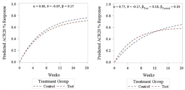
Figure 3. ACR20 response pattern according to Reeve’s model. Left panel displays a parallel curve pattern (identical slope between treatments), right panel displays a crossed curves pattern (different slopes between treatments).
a) Weighted mean approach
The weighted mean approach involves estimating the differences in response rates at each time-point alongside its standard error, and then averaging them using the inverse standard error as weight. To make inference on this weighted mean, we estimate a weighted standard error as follows:
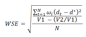
where N is the number of time-points, dt is the difference at time t, d is the weighted mean, wi is the weight for the i-th difference, V1 is the sum of weights and V2 is the sum of squared weights. Then, a confidence interval using the Normal approximation can be estimated at the prescribed confidence level.
b) GEE approach
This approach relies on estimating a GEE model for binary data using an identity link to obtain the difference in proportions across all relevant time-points alongside its confidence interval. This can be done using the following example code:
PROC genmod data = <dataset> descending;
class treatment(ref = 'Control') subjid week;
model acr20n = treatment time treatment*time/ dist = bin link = identity alpha = 0.05 cl;
lsmeans treatment/ ilink diff cl;
repeated subject = subjid / type = exch;
RUN;
Starting from the model suggested by Reeve and briefly described in Section 2, we have simulated ACR20 data using different parameter models and a varying overall sample size, ranging from 50 to 250, in order to assess the power to detect equivalence of the two alternative approaches described above.
Simulation results
In Figure 4 we report a 3D plot showing the values of the 2-norm (obtained using the trapezoidal rule rather than by numerical integration) in relation to a variety of parameter values. The shape of the surfaces suggests that 2-Norm values are more affected by the slope β (Panel A) and the differential treatment effect θ (Panel B) than they are by reference drug effect α. Moreover it also highlights, as mentioned above, that these values cannot be mapped to any useful scale in terms of equivalence margins, making them very difficult to interpret.
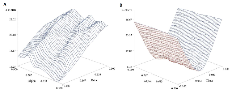
Figure 4. Estimated 2-norm values under different parameter values for Reeve’s model. Panel A is based on a fixed θ parameter (= -0.05) and panel B on a fixed β parameter (= 0.40). A sample size n of 200 was considered here for the sake of illustration.
In Figure 5 we report the power curves for the weighted mean and the GEE approach to detect equivalence between treatments in the parallel curve settings, using given values of model parameters. The figure was obtained using 500 simulated dataset and a -10% to 10% equivalence margin. The GEE approach is seen to slightly outperform the weighted mean approach, though the two curves have very similar trends.
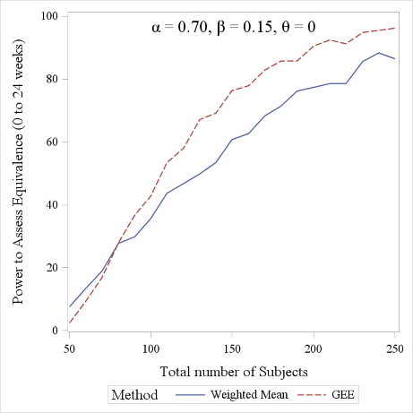
Figure 5. Power comparison between the Weighted Mean and GEE approach (range considered: 0 to 24 weeks). A 1:1 allocation ratio was considered for the sake of simplicity.
Conclusion
Whilst it is usually sufficient, for regulatory approval, to demonstrate that the difference between two treatments at a single time-point doesn’t exceed a given margin, regulators and clinicians are interested in an overall profile assessment as well. This occurs under the rationale that a drug whose beneficial effect takes considerably longer to kick in, yet with no superior effect at the end of the study, might not be a good prescribing choice. Here we have shown 3 methods to perform this ‘longitudinal’ comparison, assuming the response follows an exponential model. Notably, these are only examples, the key message being that assessing therapeutic equivalence is a complex and multifaceted task and should not be limited to a single time-point analysis.
References
- Reeve R, Pang L, Ferguson B, O’Kelly M, Berry S and Xiao W. Rheumatoid Arthritis Disease Progression Modeling. Ther Innov Regul Sci 2013, 47(6): 641-650
- Choe J, Prodanovic N, Niebrzydowski, Staykov I, Dokoupilova E, Baranauskaite A, Yatsyshyn R, Mekic M, Porawska W, Ciferska H, Jedrychowicz-Rosiak K, Zielinska A, Choi J, Rho YH and Smolen JS. A randomized, double-blind, phase III study comparing SB2, an infliximab biosimilar, to the infliximab reference product Remicade in patients with moderate to severe rheumatoid arthritis despite methrotrexate therapy. Ann Rheum Dis
- Efron B and Tibshirani RJ. An Introduction to the Bootstrap.1993, CRC Press
Quanticate's Statistical Consultants have a range of experience in supporting RA clinical trials and would be delighted to discuss your requirements and provide advice about possible ways to increase the chance of a successful study. For more information please request a consultation below.


