R Programming Datasets - Are they reliable & efficient for SAS Datasets?

R is the open source software environment and language used for data analysis and statistical computing. A great deal has already been said and written about R’s wide variety of graphical and statistical techniques. Even though R as a programming language is constantly growing in popularity in the pharmaceutical industry, it is still quite unpopular to use R in the preliminary stages of research like importing data from different sources, tidying it, calculating new variables in datasets and making other amendments available in SAS data steps.

This blog explores the ways R can come in useful as a tool for programming datasets and compares both tools in terms of performance and ease of use. It will also focus on the reliability of packages (from CRAN repository, Bioconductor and other sources) that one can use when creating and modifying datasets in R.

For most people who work with data, the start of performing exploratory analysis is a milestone of the study. Everything that needs to be done before is perceived as a sad duty or a waste of time, but it can be crucial for the quality of the whole analysis. When one works with real-world data, it can turn out to be tricky to get consistent, tidy data from the initial source collection. Cleaning, integration, transformation and reduction of data are usually performed in SAS®, the most widely used tool in the pharmaceutical industry. Even though R gains increasing popularity among programmers and statisticians working on clinical trials, especially on the production of Tables, Listings and Figures (TLFs), the focus is mainly on its graphical facilities and wide variety of statistical techniques that can be easily implemented thanks to R packages.

The aim of this blog is to show how easily dataset modifications that are usually performed with SAS data steps can be implemented in R with the use of the most reliable and popular packages. This blog will compare both tools, point out difficulties data scientists can potentially encounter when working with sets of data in R, and suggests how to overcome them. In this blog you find R usage in simulated clinical trial examples and get insight into possibilities provided by functions of the tidyverse packages.

Let's Start with the Basics

To put it in a nutshell, SAS is a high-level language and R is slightly lower-level (not low level in commonly accepted meaning though, R is counted among high-level languages) and hence equivalents of simple SAS procedures may require many lines of code, but then again, thanks to the wide variety of R packages, there are many things that can be programmed much faster in R. Beyond any doubt, SAS is more intuitive, but I personally did not notice that R is more difficult to learn, even though I started with R when I had no previous experience with data science, statistical packages or other programming languages. Using both tools at the same time is not problematic, the only thing that can be difficult for beginners to adjust to is case insensitivity of SAS and case sensitivity of R or SAS’s semi-colon which is often the first pitfall for those learning the language. In SAS, any improvements can be only added in new officially released and validated versions whilst in R the community of users add improvements quickly, but then again, improvements in R are not centrally validated and hence are not always reliable. Obviously, it is not possible to unequivocally say that R is better or worse than SAS in terms of working with sets of data, but beyond any doubt knowing R can turn out to be helpful for every SAS programmer.

It is good to know that the development of R is community-driven. The R community is noted for its active contributions in terms of creating and maintaining packages. One of the most important differences between R and SAS is that R uses main memory to store data, whilst in SAS only part of the data resides there. Nowadays, it has not so big an impact because of working on 64-bit machines, but data handling is still a reason why many users prefer to use SAS and rate it higher. Needless to say, both languages can be used in the same research and plenty of data scientists have a tendency to use these tools for that purpose. They often use SAS to get tidy data and then switch to R to make use of the graphical facilities and packages with advanced statistical techniques. It would be difficult to point out anything that can be done with the use of regular SAS language or PROC SQL that is not available in R, so why not perform the whole research in the open source counterpart of the current market leader in the pharmaceutical industry?

Everyone can easily get started with R. RStudio is an open source integrated development environment (commonly abbreviated to IDE) for R and installation of it takes a maximum of several minutes. SAS users can also use the PROC IML statement available in SAS (requires additional license though) and take the first step with R codes there. Below you can find an example of simple R code written in the PROC IML statement.

title1 j = l "Protocol: Example Study" j = r "Page 1 of 1"; 

title2 j = l "    ";

title3 "Table 1. Analysis of Covariance (ANCOVA) - leprosy treatment data" j = l; 

Generally speaking, programmers and data scientists should not encounter many obstacles when using both languages to work with data in one clinical research project. SAS datasets can be transferred to R data frames and vice versa- as R also has functions that make this possible.

Programming Data Frames in R

There are three different structures in R that store data and are somewhat similar to SAS datasets. They are regular data frames, data tables, and tibbles. Data frame is the most popular of these and most R packages use it.

In fact, this is a two-dimensional list. In general, the basic rules are the same as in SAS, all columns have to be the same length (a column length is defined once for all rows), but each can contain a different type of data. Tibble is a stricter data frame (described by its authors as “modern re-imagining of the data frame”) that forces the user to write easier to maintain and cleaner code. For instance, partial matching of column names is unavailable and warnings are generated when one tries to access the column that does not exist. Users can easily convert tables, regular data frames, matrices, or lists to tibble. Data tables can also be described as an enhanced data frame.

They are especially recommended for those who work with large data sets and want to reduce programming and computing time. Data tables are available in the data.table package, which has its own syntax for performing data modifications.

Basic Data Transformation

As a statistical programmer, I have had opportunities to work with both regular SAS data steps or procedures and SQL available via PROC SQL. After finishing one of my projects, I was asked to re-do all preliminary steps of a project with R to examine the possibility of switching permanently from SAS to this language or even to use them interchangeably and look for ways to make data tidying easier. Given below are codes with functions I used to perform the most common and basic data modifications in R followed by short descriptions.

When working on modifications of datasets, I always use the tidyverse set of packages that work together. Hadley Wickham, one of the tidyverse authors and maintainer, describes it as an “ecosystem of packages”. The tidyverse includes packages to import (e.g. readr), tidy (tidyr), transform (dplyr), visualize (ggplot2), and model data (modelr). There are also packages that enhance R’s functional programming toolkit and those designed to make working with strings much easier. In most cases packages from the tidyverse will allow you to perform all steps needed to get consistent data with derived variables.

As previously mentioned, the tidyverse contains several packages that allow users to import external files into R. For instance, the haven package can be used to import SAS files (but also those created in Stata® or SPSS®). There is another helpful package for that, sas7bdat, but big-endian files (files with values where the most significant byte is first) are not supported and hence errors can be generated. According to the specification written by an author of the sas7bdat package, it is an “experimental” function. However, in most cases, both options work fine, but the tidyverse is one of the most popular sets of R packages with a high level of reliability, so it is advisable to use the haven package instead of the sas7bdat. Moreover, reading data with the haven package will not remove labels of variables by default. Both ways to import files are shown below.

#'read' function from the sas7bdat package
demog <- read.sas7bdat("H:/rproject/project_y_r2/demog.sas7bdat")
#'read_sas' function from the haven package (part of the tidyverse)
taadmin <- read_sas("H:/rproject/project_y_r2/taadmin.sas7bdt")

If you are working with RStudio, your new data frame will appear in the Environment tab directly after importing and you will be able to check how the data looks.

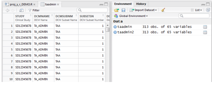
Notice that there is a Filter option which is helpful if any quick checks are needed. The data frame above has been created with use of the haven package, so labels have not been deleted and are visible below variable names.

The first steps of programming datasets in the described project required importing data from SAS files, choosing observations with valid values of one of the variables and selecting needed columns. Thanks to the dplyr package which is also part of the tidyverse it can be done in an easy way with the use of ‘select’ and ‘complete.cases’ functions as shown below. In this case, the ‘complete.cases’ function has been used to choose observations with non-missing values of the ‘DOSECUN’ variable. Notice that the same name of the dataset (‘TAADMIN’) has been used on both sides of the arrow, so the dataset will be overwritten. The arguments in the ‘select’ function is the dataset name followed by names of needed variables.

#'complete.cases' and 'select' functions from the dplyr package
taadmin <- taadmin[complete.cases(taadmin[["DOSECUN"]]), ]
taadmin <- select(taadmin, INV, PT, DCMDATE, DOSECUN, DOSETL)

Perhaps it is also worth mentioning that R has two NULL-like values, NULL and NA. NA is a logical constant of length equal to 1 which contains a missing value indicator, whilst NULL represents the null object. Some define this difference in the following way: NULL does not yield any response when evaluated in an expression and NA gives a response that is not available and hence unknown.

One of the most powerful tools of R is pipe with its widely known operator %>%. It allows the user to write code that is easier to read, understand and maintain and can be used thanks to the magrittr package. The example below shows that multiple intermediate steps of data modifications can be easily written in one line of code. The shortest possible explanation of how pipe works is that it takes output of the statement preceding an operator and uses it as the input of the next statement. When there are many commands, one can note how big the difference is in the readability of the code written with and without pipelining. For instance, calculating the Euclidean distance between two vectors (v1 and v2) can be implemented in two ways shown below.

mean02 <- as.data.frame(t(sapply(mean01, I))) 

result <- sqrt(sum((v1-v2)^2))
result <- (v1-v2)^2 %>% sum() %>% sqrt()

The ‘filter’ function used in the example below comes from the dplyr package and works similar to the ‘where’ statement from regular SAS and PROC SQL. It is important to know that even if the condition referring to a row evaluates to NA, it is dropped (unlike the sub-setting operator [condition] from the base module of R).

#'complete.cases' and 'select' functions with the use of pipe operator
taadmin2 <- taadmin %>% filter(complete.cases(taadmin[["DOSECUN"]])) %>% select(INV,
PT, DCMDATE, DOSECUN, DOSETL)

The SAS equivalent of what was done in R with the use of pipelining could look like below

data taadmin2 (keep=inv pt dcmdate dosecun dosetl flag);
set taadmin (where=(dosecun is not null));
run;

I personally prefer the syntax of R which is easily readable and shows how computations are being performed step by step. It is worth mentioning that good programming practice requires code to be easily readable also. The next step in the project was looking for the first and last observation of each patient according to chronological order. This was performed in R by the following steps:

taadmin <- taadmin[order(taadmin$PT, taadmin$DCMDATE),]
taadmin <- cbind(taadmin, flagf=0, flagl=0)
taadmin[[6]] <- (!duplicated(taadmin$PT))
taadmin[[7]] <- (!duplicated(taadmin$PT,fromlast=TRUE))

‘Order’ is available in the R base module and can be used to sort data frames by one or more columns. By default, it sorts data in ascending order, but the user can set the value of ‘decreasing' argument as ‘TRUE’ or add minus sign before sorting variable to order values descending. ‘cbind’ and ‘rbind’ are methods used to combine objects by columns or rows, respectively. They are both useful when one wants to add observations or variables to a data frame. In fact, using ‘cbind’ function and initializing flags values are not necessary before determining the first and last observations.

Each can also be done in one line, e.g.

taadmin$flagf <- (!duplicated(taadmin$PT))

Using the ‘duplicated’ function from the R base module is a good way to find first and last observations for all patients. Note that data had been previously sorted chronologically. The exclamation mark before the function forces it to return TRUE if the observation is first and FALSE otherwise instead of returning TRUE in case of duplicated values like it does by default. Setting ‘fromlast’ argument value to TRUE helps find last observations. Generally speaking, performing such operations look very similar in SAS. In this case, the advantage of SAS are variables ‘first.’ and ‘last.’ that assign the value of 1 for the first and last observation respectively in a ‘by’ group.

proc sort data = taadmin2;
       by pt dcmdate;
run;

data taadmin3;
       set taadmin2;
       by pt dcmdate;
       flagf=0; flagl=0;
       if first.pt then flagf=1;
       if last.pt then flagl=1;
run;

The next task was to calculate the sum of the ‘DOSETL’ variable for each patient. There are several methods that allow us to do this. One can use the ‘aggregate’ function available in the automatically installed stats package or the ‘group_by’ function from the dplyr package which may resemble the syntax of PROC SQL. Moreover, the ‘aggregate’ function can be implemented in two different ways (examples below). All three approaches presented below can be used inside a pipeline. The ‘group_by’ function from the dplyr package can be helpful in multiple situations, e.g. for selecting first, last, or even n^th observation of a group, so could replace the ‘duplicate’ function used in a previous step.

#first approach gives calculated variable ‘x’ name by default
taadminagg <- aggregate(taadmin$DOSETL, list(taadmin$PT), sum) %>% filter(x>0)
#alternative approach with use of aggregate function
taadminagg <- aggregate(DOSETL ~ PT, taadmin, sum) %>% filter(DOSETL>0)
#third approach- dplyr package
taadminagg <- group_by(taadmin, PT) %>% summarise(sum = sum(DOSETL)) %>% filter(sum>0)

The inherent part of any study is acquiring information from different datasets and summarizing it in one table. There are several types of merging data that can be performed with the use of joins in PROC SQL or the ‘merge’ statement in a data step. The R language is no different and makes it possible to use the ‘merge’ function (from the R base module) and specify arguments’ values to achieve an expected result. The examples below show how to perform the ‘left join’ equivalent with the ‘ALL.X’ argument equal to ‘TRUE’. The first example refers to the situation when joining variables have the same name in both data frames. In the second example, we want to join data frames with the use of two different variables from each data frame. To perform this, we need to assign vectors with variable names to ‘BY.X’ and ‘BY.Y’ arguments. The last line of code allows us to merge data frames by one variable from each data frame- the ‘PT1’ variable from the ‘TAADMIN’ data frame and the ‘PT2’ from the ‘TAADMINGR’ data frame.

#left join equivalent- merge function
taadmin <- merge(x = taadmin, y = taadmingr, by = "PT", all.x = TRUE)
taadmin <- merge(x = taadmin, y = taadmingr, by.x=c("PT1","DT1"), by.y=c("PT2","DT2"),
all.x = TRUE)
taadmin <- merge(x = taadmin, y = taadmingr, by.x="PT1", by.y="PT2", all.x = TRUE)

The code above shows how easily merging data frames can be done in R. Inner join is the default type, but ALL, ALL.X and ALL.Y arguments allow users to perform different merging types. There is another way of joining tables using the well-known dplyr package and a specific function for each type. It has a syntax looking very familiar to PROC SQL users. The examples are shown below. They refer to three cases described and performed with the use of the ‘merge’ function before.

#one of the merging functions from the dplyr package
taadmin <- left_join (taadmin, taadmingr, by = PT)
taadmin <- left join (taadmin, taadmingr, by = c("PT1" = "PT2"))
taadmin <- left join (taadmin, taadmingr, by = c("PT1" = "PT2", "DT1" = "DT2"))

Do it smart with DPLYR

It is easy to spot that the dplyr package from the tidyverse is a great tool for working with data frames and data transformation in general. Obviously, it can do much more than what has been shown above. Beyond any doubt, it is worth taking the time to describe dplyr functions more precisely. Similar to SQL, there are six basic verbs in the dplyr package: arrange, filter, group_by, mutate, select and summarise. Since many of them have already been used in the code examples above and their names explain a lot, there is no need to describe all of them separately.

This section shows how to perform useful data manipulation steps with the use of the dplyr package, write code that is easy to understand and avoid too much typing.

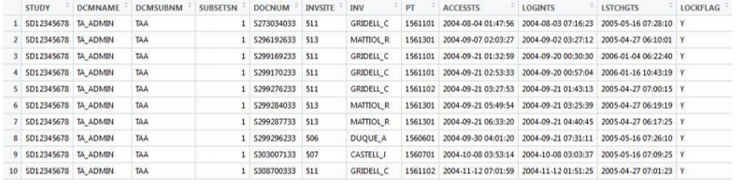
As stated previously, ‘select’ is one of the basic dplyr functions. What I personally like the most, in that it is allowed to use colons and regular expressions to choose columns we want to display. Suppose we have a dataset like that shown below, and we want to select only the first four variables and those that start with the letter “L”.

To do it in R with the use of the ‘select’ function from the dplyr package, it is enough to write

taadmin2 <- select (taadmin, STUDY:SUBSETSN, starts_with("L"))

‘starts_with’ is not the only argument that can be specified to determine what observations are to be selected. There are also ‘ends_with’, ‘matches’ and ‘contains’. It is even possible to use them all in one line of code multiple times to specify many patterns to match with.

The other term ‘summarise’, is the most useful when dealing with grouped data, so it is usually used in pipeline statements. Suppose we need to calculate an average dosecun per patient and sort the data frame in descending order. With two basic functions from the dplyr package, it can be done in one line of code.

taadmin2 <- taadmin %>% group_by(PT) %>% summarise(avg_d=mean(DOSECUN)) %>%
arrange(desc(avg_d))

If there is a need to apply the same function (e.g. ‘min’, ‘max’, ‘mean’, number of unique values or even as mentioned before the value of the n^th observation for each group) to multiply columns, ‘summarise_all’, ‘summarise_at’ or ‘summarise_if’ can be used, which is extremely helpful (they refer to all variables, to a selection of variables and variables that meet the specific condition, respectively). All three variants are available for use with the ‘mutate’ function, useful for applying a transformation of variables. The function ‘arrange’ is equivalent to SAS PROC SORT or the already mentioned ‘order’ function from R base module and can be used as a statement in a pipeline.

With the dplyr package the programmer can also use window functions. Submitting the lines shown below will create a data frame with two columns: ‘PT’ and ‘DOSECUN’. It will contain patient number and the three highest values of dosecun for each patient.

taadmin2 <- taadmin %>% group_by(PT) %>% select(DOSECUN)
%>% filter(min_rank(desc(DOSECUN)) <=3) %>% arrange(PT ,desc(DOSECUN))

The same result would be given using a wrapper that uses ‘filter’ and ‘min_rank’ functions and is also available in the dplyr package.

taadmin2 <- taadmin %>% group_by(PT) %>% select(DOSECUN) %>% top_n(3)
%>% arrange(PT ,desc(DOSECUN))

Using ‘min_rank’ without adding ‘desc()’ or setting a negative number for a ‘top_n’ function argument would lead to displaying the bottom rows.

Many more useful window functions are available in the dplyr package, e.g. looking familiar for SAS users and self-explanatory ‘lag’ or ‘row_number’ functions. It is also worth mentioning that the ‘lead’ function is available thanks to the dplyr package. It can be used to find the “next” value of a particular variable in the data frame. That is extremely useful compared to SAS, where there is no single function that looks ahead and instead requires multiple steps or reading the dataset in multiple times (e.g. sorting in reverse order and using the ‘lag’ function).

Performance of R Programming Datasets

It has already been mentioned that data handling is one of the most crucial differences between SAS and R. By default, R loads all data into memory, whilst SAS allocates memory dynamically and handles large datasets better. I personally did not encounter the problem when data was too large for R and hence I have not needed to look for ways to overcome that, but I did notice how many statistical programmers point out handling big data as one of the biggest R weaknesses. A great source of knowledge regarding improving performance of R code is the chapters Measuring Performance and Improving Performance from the book Advanced R written by Hadley Wickham, Chief Scientist at RStudio. Firstly, it is usually possible to reduce the size of the file before loading it into R. If it is not the case, one of the methods that can allow the programmer to work with big sets of data in R faster is using data tables instead of data frames. The other way to make R work faster is code vectorizing. In general, R code based on loops performs slower. Obviously, vectorizing is not only for avoiding loops, but it can be helpful too. Vectorized functions and loops inside them are written in C language, which is really important for the performance of the code-loops in C are faster.

When considering the performance of R, it is advisable to take implementations into account. GNU-R is the most popular implementation, but there are many other that perform much better.

Finally, it comes as no surprise how vital the community of users are as they work tirelessly on improving R’s performance with large sets of data, and there is a lot of interest around how to handle it. Programming Big Data with R, often abbreviated to pbdR, is a series of packages designed for distributed computing and profiling in data science. Another helpful tool is RHadoop, a set of R packages that allow users to manage and analyze data with Hadoop. Additionally, another method of improving performance, parallel computing, is also possible in R thanks to several packages, e.g. doMC, Rmpi or snow. 

Does R Stand For Reliability?

The reason why SAS is generally preferred by many programmers and companies is its high-level quality control. R provides absolutely no warranty and users need to be more careful. As I stated previously, the strength of R is its community and a wide variety of packages. R Packages are shared most often via CRAN, Comprehensive R Archive Network, but there are also many of them on GitHub, RForge or BioConductor.

In the pharmaceutical industry, it is necessary and essential that the research is secure, reproducible and reliable, so acquiring packages is crucial. Each company or a single programmer should thoroughly consider what sources R packages should be downloaded from. The most reliable repository of packages is CRAN. GitHub is mostly under the control of individual developers. Packages change over time and what works today, may not work tomorrow, they also can be removed. Obviously, even GitHub packages have standards, but those on CRAN and BioConductor are more formal. Especially important is that these sources preserve older source versions of packages in their archives so that any package version can be rebuilt if needed, which alleviates one aspect of “reproducible”.

All in all, the decision of what packages are trustworthy and can be used to process data will be always on the part of the particular company. Everybody should be aware of the fact that the U.S. Food and Drug Administration (FDA) allows the use of R and validation coverage is entirely up to the company submitting to the FDA. If you are sure that the tool and its packages you are using are reliable, there is no contraindication to its use. The document “R: Regulatory Compliance and Validation Issues. A Guidance Document for the Use of R in Regulated Clinical Trial Environments” published by The R Foundation for Statistical Computing can be helpful, but it is only applicable to base module and recommended packages, so, as of this writing, 29 packages in total. Neither base nor recommended packages sections include the tidyverse set.

Beyond doubt, validation of software is time-consuming and challenging, but R can be validated
just as well as commercial software, there are companies that offer validated versions of R. Highly recommended is the setting up of the company’s own repository that can be validated, version-controlled and archived if needed. It can contain reliable packages that turned out to be useful in clinical trials in the past. It is important to remember that users can check the source codes provided for all packages to base the decision about using package or not on what the source code contains. Obviously, however it requires proficiency and much experience in R to make that judgement. There are also several paid methods of assuring enhanced control and reducing the risk presented by R as an open-source software, e.g. ValidR. If you consider writing your own packages to use them in clinical trials, I recommend the book “R packages” by Hadley Wickham.

Conclusion

To sum it up, R is a friendly tool that can be used not only for statistical inference, modeling and creating advanced plots, but also for data tidying, modifying and standardization. It could be backbreaking to look for something that can be done with the use of regular SAS DATA STEP or PROC SQL and is not available in R. Thanks to a large number of packages maintained by the community and experienced developers, many things can be done in different ways. There are many R packages that have been thoroughly tested and programmers from the pharmaceutical industry use them in clinical trials with no worries or concerns about reproducibility, reliability and correctness of results.
It is important to remember that R is developing at an extraordinary speed and we can expect that this tool will be even more useful and user-friendly in the future. I personally recommend using R for programming datasets. It can be a great replacement for paid software, but it can also be used together with SAS even in one clinical research project.

Turn your validated trial data into interpretable information ready for biostatistical analysis. Using R Programming or SAS, Quanticate can help you better understand the effect of your investigational product and it’s safety and efficacy against your trial hypothesis with the creation of analysis datasets and production of TLFs. Submit a RFI and member of our Business Development team will be in touch with you shortly.