Using R Programming for Clinical Trial Data Analysis

The use of R programming in clinical trials has not been the most popular and obvious, despite its recent growth over the past few years, its practical use still seems to be hindered by several factors, sometimes due to misunderstandings, (e.g validation) but also because of a lack of knowledge of its capabilities. Despite these bottlenecks, though, R is doubtlessly creating its own (larger by the day) niche in the pharmaceutical industry.

In this blog we will see how R can be used to create TLFs much like the current combination of PROC REPORT/PROC TABULATE and the ODS currently does, thus showing its power and capability to play an important role in our industry in the years to come, not as a replacement for, but rather as an alternative option to SAS®.

Watch our statistical consultant explore the most suitable manner of creating TLFs, be it R or SAS in the presentation below:

R versus SAS for TLFs

Everyone involved in any capacity in clinical trials reporting is aware of a sort-of self-proclaimed truth that can be broadly summarized as ‘Thou shall not have any software other than SAS’. Whilst this has been practically true for quite some time, somehow based on the misconception that regulators ‘strictly’ requested submissions to be made using SAS, other players have started to make their appearance in the pharmaceutical industry arena and draw attention of statistical programmers and statisticians alike. The most famous of these is most certainly the open software R, which has a long track record of usage in academia, both for applied and theoretical statistical research, and has been used to date also in the pharma industry, though its adoption in submissions has been hindered by the above described misconception.

Setting aside the validation part of the flow (which is a current hot area of discussion when it comes to R but will not be discussed here), moving from SAS to R for such a consolidated task as Tables, Listings and Figures (TLFs) creation does require some re-thinking. How the actual reporting works is a challenge as there is not a direct PROC REPORT counterpart that can be used straight away to export results to an output file, but that is the only real challenge. Since in most cases the efficiency with which a software can perform a task heavily depends on the ability of the end-user to exploit all of its features, using R efficiently (the same way we’ve been doing with SAS for quite a while now) simply implies getting used to it and getting to know all the ‘arrows in its quiver’ available to achieve a goal. In this blog we will first see how a specific TLF (including both summary and analysis sections) is usually generated in SAS and then we’ll see how the same table can be created and reported using R.

Generating an Analysis Table using SAS

No matter the software we use, i.e. SAS or R, to create a table or a listing (and to some extent also a figure) we’ll have to manipulate a source dataset (or more than one) to create a dataset/data frame that to a certain extent mirrors a given table specification, and then feed this dataset to a procedure (in SAS) or function (in R) that ‘translates’ the dataset into a neatly formatted table.

However, whilst this workflow appears rather slim, there’s a variety of decisional branches that need to be considered before choosing how to practically implement it. One key thing to decide is the actual format of the output table or listing: in many cases tables are created as plain text documents (.txt) which are then collated to a Word or PDF document using tools that are often external to the statistical software (e.g. VBA macros, UNIX scripts), but other viable options include either creating tables as Rich Text Format (.rtf) or .doc/.docx files to read into Microsoft Word straight away (and also in this case collation for reporting purposes is done outside of the software) as well as Portable Document Format (PDF) or html files.

For the sake of illustration, we will use data from a study on leprosy treatment described in Snedecor and Cochrane seminal Statistical Methods book ^[1]. The data has been arranged as a 3-columns dataset: Drug, Baseline and End of Treatment measurement (similar to a very simple CDISC ADaM BDS dataset, without subject ID as it’s not relevant for the example).

The goal is to produce a table so that for each of the 3 treatment arms, basic summary statistics are displayed as well as a section with a statistical analysis that compares drugs A and D to drug F (the control arm). If we wanted to create this kind of table using SAS we’d most likely use a combination of PROC MEANS/PROC SUMMARY/PROC UNIVARIATE for the first two sections (depending on our preferences or existing company-specific standard macros) and e.g. PROC GENMOD/PROC MIXED for the analysis section (again, depending on our preferences, though in this simple example there’s no clear advantage in using one vs the other) coupled with some data wrangling to put results together and have them in a dataset ready to feed into PROC REPORT, as in Figure 1 below.

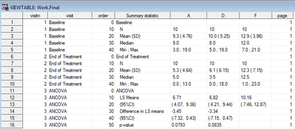
Figure 1. SAS dataset to create ANCOVA table

Whichever the output destination, the core PROC REPORT specifications will be pretty much the same, the main difference being the need to add some style commands when e.g. outputting to RTF to ensure the specifications are followed. The syntax for a plain text file here would look as follows:

title1 j = l "Protocol: Example Study" j = r "Page 1 of 1";

title2 j = l "    ";

title3 "Table 1. Analysis of Covariance (ANCOVA) - leprosy treatment data" j = l;

proc report data = final headskip headline formchar(2)='_' spacing = 0 nowd center; column ("             " page visitn order _label_ A D F);

define page / noprint order; define visitn / noprint order; define order / noprint order;

define _label_ / "" display width = 33 flow;

define A / "Drug A" display width = 22 center flow; define D / "Drug D" display width = 22 center flow; define F / "Drug F" display width = 22 center flow;

break after visitn / skip; compute after page;

line @1 "&line.";

line @1 "Generated on %sysfunc(date(),date9.) (%sysfunc(time(),time5.))"; line @1 "by &dir.table1.sas";

endcomp;

run;

The nice thing about the above commands is that the input dataset matches the shells only partially and full adherence can be obtained by using the plethora of built-in options that PROC REPORT features. Finally, in order to have the above sent to a .txt file we can wrap the PROC REPORT call between two PROC PRINTTO calls (the first starting printing to an output file, the second resuming printing to SAS listing), whereas for a .rtf file we could use the ODS RTF command (syntax skipped here), and for a .doc/.docx Word file the most recent addition ODS WORD (though the author hasn’t had the chance to use it yet). Figure 2 shows the resulting .txt file using the above PROC REPORT syntax.

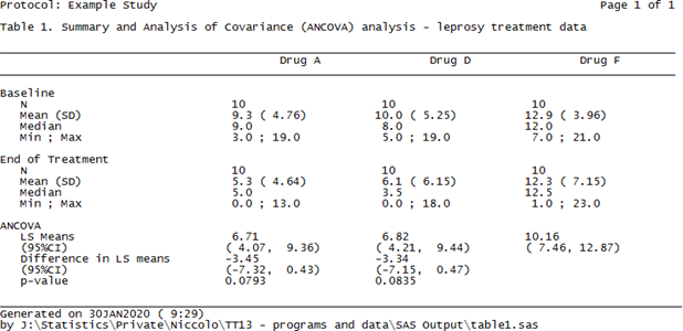
Figure 2. A .txt. table created using PROC REPORT

Generating an Analysis Table using R

A criticism often directed at R, in particular from die-hard SAS users, is that it’s too dispersed, with too many packages that quite often do the same things but provide results in a somehow inconsistent and incoherent manner. This can in fact be a great advantage when it comes to manipulating data frames to calculate simple summary statistics as well as fitting complex statistical models. Before moving onto the reporting bit, we will see how the summaries and ANCOVA section of the table can be quickly created using R to illustrate how this flexibility can be leveraged to achieve our purposes.

The summary statistics sections of the table are usually created in SAS by passing the source dataset to one of PROC MEANS, PROC SUMMARY or PROC UNVARIATE and the resulting dataset has to be re-formatted for our purposes. In order to do the same in R we can either manually write a function that calculates each summary and then arrange it, using e.g. tapply or by:

mean01 <- by(ancova, ancova$Drug, function(x){ means <- colMeans(x[,2:3])

})

mean02 <- as.data.frame(t(sapply(mean01, I)))

Note in the above the second and third column in the data are the baseline and post treatment values, respectively. Also we can re-arrange the source data in long-format (i.e. adding numeric (VISITN) and character (VISIT) variables identifying the time-point being summarized and then rely on one of the many wrapper functions such as ddply from the plyr package to calculate everything for us and put it in a nicely arranged dataset (similar to a PROC MEANS output):

descr01 <- ddply(ancova02, .(visitn, visit, Drug), summarize,

n      = format(length(Drug), nsmall = 0),

mean   = format(round(mean(aval), 1),

nsmall = 1), sd   = format(round(sd(aval), 2), nsmall = 2),

median = format(round(median(aval), 1), nsmall = 1),

min  = format(round(min(aval), 1), nsmall = 1), max  = format(round(max(aval), 1), nsmall = 1))

This latter option was chosen here for it returns a readily usable data frame with already formatted summary statistics that then needs to undergo the usual post-processing steps to obtain an object that mimics the table shell. By using some functionalities of the tidyr package this can be easily achieved with no more programming efforts than it would using SAS.

The analysis section part can then be programmed in its core contents in a very compact manner:

model <- lm(PostTreatment ~ Drug + PreTreatment, data = ancova)

lsmeans <- emmeans(model, specs = trt.vs.ctrlk ~ Drug, adjust = "none")

lsm_ci <- confint(lsmeans)

The first line fits a linear model to the data; the second creates a list that contains two elements, the Least Squares (or Estimated Marginal, in the emmeans package) Means for each level of the factor ‘Drug’ alongside their 95% CI and their difference using a control reference class (in this case drug F); the third line is needed to create an object identical to the one created above that however stores the 95% CI for the differences instead of the p-value testing the hypothesis that the differences are equal to 0 (since the shell requires both). Once this section is post- processed using whichever combination of SQL-like language using sqldf or base R functionalities, we end up having the following data frame:

Creating this dataset took more lines of codes with SAS compared with R after excluding comments and blank lines as well as ‘infrastructure’ code (i.e. setting of libnames and options for SAS and loading of required libraries for R), and using a consistent formatting style (although R functions lend themselves more to compactness, i.e. one line of code for a function, much more than what SAS procedure statements need for ease of reading). Whilst this per se does not necessarily mean that R is more efficient than SAS (runtime on a large dataset or a more complicated table would be a much better indicator), it suggests that R offers an elegant and compact way of summarizing and analyzing data which is perfectly comparable to what SAS offers (and this is by no means a small thing!).

Notably, the first difference compared to SAS is that here we haven’t included the sorting variables VISIT/VISITN/ORD that were available in the SAS final dataset, the reason being that since they’re not going to be in the printed report there is no point in having them in (since it would be redundant including them only to have a selection that filters them out). Linked to this, the white lines between each section have been effectively added in as empty rows to mimic the table shell, something that in SAS we accomplished via the SKIP option in a BREAK BEFORE command. The general ‘take-home’ message is that the data frame to report needs to look exactly like the resulting table, and that includes eventual blank lines, order of the rows, ‘group’ variables (e.g. subject ID in listings where only the first occurrence row-wise is populated and the other are blanks).

At this point, having created the dataset in a rather simple manner, is it as simple to export it for reporting? As mentioned in the Introduction, there’s no R version of PROC REPORT however there are tools and functions that allow this task to be achieved using a comparable amount of programming as SAS with comparable quality. Whilst there are many options to achieve this, not all of them are as seamless to use as PROC REPORT and the resulting output is sometimes not fully fit for purpose. The combination of the officer and flextable packages, nevertheless, provides the user with a rich variety of functionalities to create nice-looking tables in Word format in a flexible manner.

The first step is to convert the data frame to report into an object of class flextable using the flextable function and then apply all styling and formatting functions that are needed to match the required layout. One useful feature of this package is that it allows the use of the ‘pipe’ %>%, a very popular operator that comes with the magrittr package and allows a neater programming by concatenating several operations on the same object. This translates in the below syntax:

summary_ft <- flextable(summary05) %>%

width(j = 2:4, width = 2) %>% width(j = 1, width = 2.5) %>%

height(height = 0.15, part = "body") %>%

align(j = 2:4, align = "center", part = "all") %>% align(j = 1, align = "left", part = "all") %>%

add_header_lines(values  =  paste("Table 1. Summary and Analysis of

Covariance (ANCOVA) analysis - leprosy data", strrep(" ", 30), sep = "")) %>%

           add_header_lines(values = paste("Protocol: Example study", strrep(" ", 93), "Page 1 of 1", sep = "")) %>%

           add_footer_lines(values = paste("Generated on ", Sys.time(), " by ", work, "Table1.R", sep = "")) %>%

hline_bottom(border = fp_border(color = "black"), part = "body") %>%

hline_bottom(border = fp_border(color = "black"), part = "header") %>% border_inner_h(border = fp_border("black"), part = "header") %>%

hline(i = 1, border = fp_border("white"), part = "header") %>% font(font = "CourierNewPSMT", part = "all") %>%

fontsize(size = 8, part = "all")

One great advantage of many functions within flextable is that they can be applied only to a subset of rows and/or columns by using standard R indexes, as we have done above to specify different column widths and alignments. The actual reporting to a Word document is done using the read_docx and body_add_flextable functions from the officer package: the first one opens a connection to a reference document (that in our case has been set to have a landscape orientation, as common for TLFs) and the second adds the flextable object created above to the document. The actual reporting is then done using the standard print function:

doc <- read_docx("base.docx") %>% body_add_flextable(value = summary_ft)

print(doc, target = "Table1.docx")

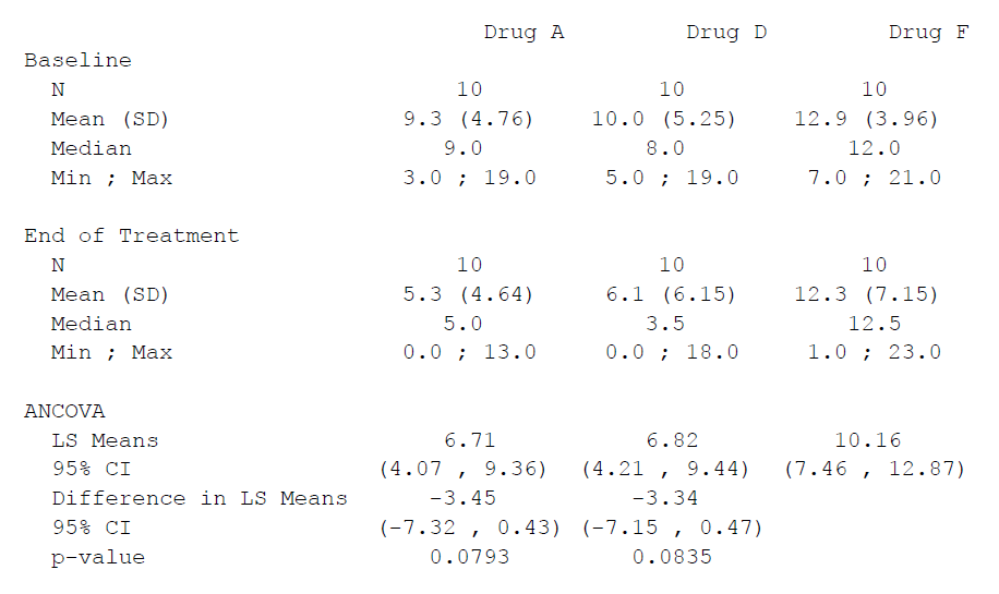
The resulting output is displayed in Figure 3 below.

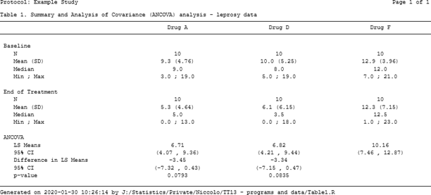
Figure 3. A .docx table file created using flextable and officer

In the above program there are a few things worth mentioning before we do an actual compare with SAS:

• the two add_header_lines calls are in a somewhat reverse order since we specify the table title before the so- called page header, but that’s because the function allows to place extra lines either at the top of the header (as default) or at the bottom, and by doing as above we first write the table title above the table, and then above the title we write the protocol name and the page number;
• the horizontal lines in the header need to be sorted out in a slightly convoluted manner: the second hline_bottom function call adds the line under the column names, the border_inner_h call adds horizontal line between all rows of the header, however since we don’t want any line to be shown between the page header and the table title we need an hline call that applies a white border at the bottom of the first header row, resulting in the table shown above;

• the result of Systime() is slightly different from SAS.

As introduced at the beginning of this blog, the reporting of Tables using R is a conceptually different process compared to SAS, however we can see that the key options that exist in PROC REPORT also exist in the flextable package, as mentioned in Table 1. There are other features (e.g. the possibility to change font, font size, etc.) that can be mapped between the two software, but those mentioned below cover the most important ones.

Table 1. Key reporting features – comparison between PROC REPORT and flextable

One specific mention is needed for the last two rows here, i.e. the chance to ‘break’ the table in different ways, either by adding blank lines between rows or by moving to another page. Fixing the first issue in R is relatively easy, as we mentioned before, whereas for the second one a different approach needs to be taken that involves writing a general function that iteratively prints pages to the reference Word document and then adds page breaks. To do this we first need to create a variable page (as we’d commonly do in SAS if we wanted to avoid odd page breaks), and then the function could look as follows:

page.break <- function(data, pagevar = "page"){

 ## Identify which variable stores the page number and how many pages

npage <- 1:max(data[,pagevar])

which.pg <- which(names(data) == pagevar)

## Define the flextable object separately for each page

for (i in npage) {

## Create the Page x of y object for the title and identify which rows to display based on page number

npg <- paste("Page", i, "of", max(npage), sep = " ") rows <- which(data[,which.pg] == i)

#flextable object definition (use the npg object to ensure the correct Page x of y header line is added

## Print the object out: if it is the first one add to base.docx otherwise add to the document with previous pages printed

if (i == 1) {

        doc <- read_docx("base.docx") %>% body_add_flextable(value = summary_ft)
fileout <- "Table1.docx" print(doc, target = fileout)

} else {

doc <- read_docx("Table1.docx") %>% body_add_break() %>% body_add_flextable(value = summary_ft)

fileout <- "Table1.docx" print(doc, target = fileout)

}

}

}

Once a page variable is added to the reporting dataset to have the ANCOVA section displayed on a separate page and the above function is applied, the result is the one displayed in Figure 4 (the actual spaces between tables have been reduced to fit this blog).

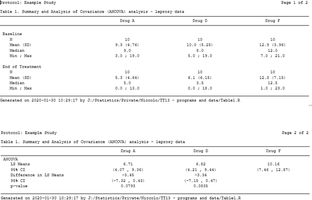
Figure 4. Multipage table using flextable and officer

The only drawback with the above is that it implies having a page variable that correctly splits rows such that when printing there’s no overflow to the next page, although this might reasonably be an issue only with long tables such as Adverse Events or listings). In general, anyway, the two packages combined offer a great degree of flexibility that allows one to reproduce a table as with SAS using a somehow more explicit report definition compared to PROC REPORT, and the actual amount of programming required is similar to SAS.

Can R Rival SAS in TLF Creation?

In the introduction we clearly stated that moving from SAS to R for TLFs implies some rethinking of the way we approach clinical trial reporting. Whilst this is indeed true, as the previous section has shown, it is important to understand that this re-thinking is in fact only minimal and somehow superficial: we’ll still be creating output datasets that other programmers will try to match on (using either all.equal or compare_df) and then exporting this to a suitable document outside of the statistical software. This being the case, the only question worth asking is ‘Why?’

In the author’s view there are many answers to this question:

• R is, as we showed, incredibly flexible: if the existing methods do not fit our purposes we can easily tweak them to do what we need (see the page.break function example). In SAS, this is not always that straightforward;
• The actual programming effort is not largely different to SAS, considering that most low-level programming is often done by standardized macros that could well be replaced by R functions;
• The collection of packages in the tidyverse now make it very easy to manipulate data frames and to perform transforming operations (e.g. transpose long-to-wide and vice versa) with very simple and compact code. Base R is still an excellent resource, of course, but for the example in this blog we managed to transpose a dataset with one simple line of code using either the gather or the spread functions from tidyr;
• In SAS there’s PROC SQL, in R one can use either the sqldf or RSQLite package, depending on preferences, so this one’s covered as well;
• The main reason (for the author) is the immense breadth of statistical methods and procedures available in R compared to SAS: mixed models, survival analysis, parametric and non-parametric tests, and many others. All these are readily available and have contributions from some of the most senior members of the R community (if not some of the main experts on the topic in the world). Plus, computationally intensive techniques (such as bootstrap or permutations) can be implemented in a more intuitive manner than with
  
  

There are certainly some cases where attempting to recreate SAS results using R and vice versa has generated more than one migraine, but in most cases this occurs because the assumptions and default implementations differ (e.g. the optimization method for a given regression) rather than because of real differences. Many of these have been documented on the internet in mailing lists and help pages, and no doubt that the more the industry starts making more consistent use of R more scenarios will emerge, thus prompting better knowledge of both software.

Conclusion

The uptake of R as software of choice within pharmaceutical companies and Contract Research Organizations (CROs) is something that many doubted to see during their lifespan, however things are rapidly moving even in the pharmaceutical industry. Nevertheless, many misconceptions about R still exist, not least whether it’s a tool suitable for creating submission-ready deliverables such as TLFs. In this blog we have seen that R can be an extremely powerful tool to create Tables and Listings using the officer and flextable packages and tools already available (and for great figures ggplot2 is available), and that by leveraging its high flexibility it is possible to obtain high- quality results with comparable efficiency and quality to standard SAS code.

All in all, the current R vs SAS debate is not fair: SAS has been used in the industry for decades now and its pros and cons are our bread and butter now, but the same can’t be said about R which is often met with prejudice due to its open-source nature. Hopefully the above example and considerations have provided a different angle to this quarrel and why it does not need to be a quarrel at all.

Turn your validated trial data into interpretable information ready for biostatistical analysis. Using R Programming or SAS, Quanticate can help you better understand the effect of your investigational product and it’s safety and efficacy against your trial hypothesis with the creation of analysis datasets and production of TLFs. Submit a RFI and member of our Business Development team will be in touch with you shortly.

References

[1] Snedecor GW, Cochran WG. Statistical Methods, sixth edition. Ames: Iowa State University Press

Appendix

Overview of the R packages used in this blog. 

https://cran.r-project.org/