
Challenges of Multiple Endpoints
Testing multiple endpoints in clinical trials presents a range of challenges that must be carefully managed to ensure reliable and interpretable conclusions. These challenges include:
1. Type-I Error InflationWhen multiple hypotheses are tested, the overall probability of false positives increases. For instance, conducting two tests at a 5% significance level raises the Family-Wise Error Rate to nearly 10%, undermining the robustness of any claims about treatment effects. This inflation necessitates statistical adjustments to maintain the integrity of findings.
Beyond the inflation of Type-I error, testing many endpoints can exacerbate the risk of spurious results. Without proper correction methods, the likelihood of incorrectly rejecting at least one null hypothesis grows with the number of tests conducted.
Many endpoints interrelated, particularly in settings involving biomarkers or composite measures. This correlation complicates the interpretation of treatment effects, as changes in one endpoint may drive similar trends in others, making it difficult to attribute effects to specific factors.
Determining the relative importance of endpoints can be subjective and context dependent. In some cases, regulatory or clinical priorities may emphasise specific outcomes, while other scenarios might require a broader perspective. Striking this balance is essential to ensure meaningful analyses.
A treatment may improve some endpoints while adversely affecting others, complicating the overall assessment of its benefit. For example, a drug might reduce disease severity but increase adverse event rates, requiring careful consideration of the trade-offs.
To address these challenges, researchers employ various statistical techniques. Traditional methods like the Bonferroni correction and Holm’s procedure help control error rates but often focus on individual endpoints, which may limit their utility in broader analyses. In contrast, advanced methods such as the Global Statistical Test (GST) offer a unified framework for evaluating multiple endpoints simultaneously. The GST is particularly useful in exploratory studies or early-phase trials, where the goal is to assess collective trends across correlated variables rather than isolate individual effects.
By carefully addressing these challenges, researchers can improve the reliability and interpretability of their findings, ensuring that multiple endpoints are analysed with rigor and precision.
What is the Global Statistical Test (GST)?
The Global Statistical Test (GST) introduced by O’Brien in 1984 [1] is a multivariate analysis method that evaluates a treatment’s overall efficacy across multiple outcomes by mapping a multivariate problem onto a univariate scale, so that subsets of variables can be assessed as a whole and a single probability statement (a p-value) can be estimated for each subset. The method is very flexible and in its simplest formulation is completely non-parametric since it’s based on ranks, however parametric versions based on Ordinary or Generalised Least Squares also have been proposed [1, 2]. the Ordinary Least Squares (OLS) applies equal weights, making it straightforward but potentially sensitive to correlations between endpoints, whereas Generalised Least Squares/Modified Generalised Least Squares (GLS/MGLS) accounts for correlations between endpoints by assigning weights based on the covariance matrices, which improves handling of multivariate data.
Advantages of the Global Statistical Test
The GST provides several benefits that make it an attractive choice for trials with multiple endpoints:
1. Whole Study Approach
The GST evaluates all endpoints together, offering a comprehensive perspective on treatment efficacy. This global approach is particularly useful in diseases with multidimensional impacts, such as Parkinson’s Disease or asthma.
2. Enhanced Power
By leveraging the inherent correlations among endpoints, the GST often achieves higher statistical power compared to traditional methods like Bonferroni correction, which can be overly conservative.
3. Flexibility
The GST is versatile, accommodating both parametric and non-parametric data and handling endpoints measured on various scales, such as continuous or ordinal measurements.
4. Error Control
The GST controls the type-I error rate without the need for stringent adjustments that reduce power, such as those required by Bonferroni or Holm’s methods, thereby preserving statistical power.
5. Transparency
Unlike composite endpoints, which obscure individual contributions, the GST retains the integrity of each endpoint while providing a global assessment.
6. Clinical Relevance
The GST reflects the real-world impact of treatments, making it ideal for exploratory studies, early-phase trials, or conditions where the focus is on overall improvement rather than isolated outcomes.
Applications of the Global Statistical Test
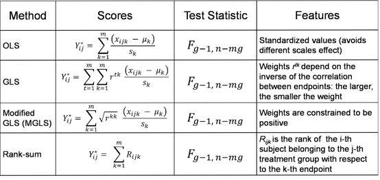
Below is a closer look at how to apply the GST, followed by a detailed example. The GST is made of up a formula where we can let g be the number of treatments, m the number of endpoints, μjk , σjk and λjk the mean, standard deviation and effect size for the j-th treatment and k-th endpoint, where 𝜆𝑗𝑘= 𝜇𝑗𝑘/𝜎𝑗𝑘. If all these treatment effects are the same across endpoints, then the problem can be simplified to a univariate one by creating convenient subject-specific scores that can then be analysed by means of common ANOVA models.
In Table 1 we summarise what these scores look like for each approach, following the notation in [3]. An interesting feature of both GLS and MGLS, which makes them particularly appealing in a number of applications, is that the correlation between endpoints is factored in the score and it down-weights the contribution of a non–independent endpoint.
Table 1: Summary of GST methods
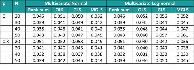
The characteristics of these methods (type I error control and power) were assessed via simulations (as in [1]). In terms of Type I error, we simulated data from 3 covariates with common and constant correlation ρ (=0 or 0.3), equal means and varying sample size (N = 20, 30, 40, 50), sampling from either a multivariate normal or a multivariate log-normal. Results are displayed in Table 2 below, and they show that overall type I error is controlled at the 5% level, the rank-sum method being the most conservative one across many scenarios, and the MGLS outperforming other methods for log-normal positively correlated samples.
Table 2: Type I error for GST methods, varying sample size and constant correlation
(1000 simulations)
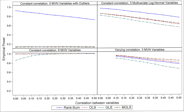
In terms of power, results in Figure 2 suggest that the non-parametric GST is more powerful when the data follow a strictly non-Normal distribution (e.g. log-normal) or in presence of outliers, whereas MGLS outpowers all other parametric options across all scenarios investigated (and the non-parametric one when data where from a pure multivariate Normal distribution). Also, the higher the correlation the lower the power.
Figure 1: Empirical power over 1000 simulations, N = 50, µA = (13, 15, 16) and µB = (13, 14, 13) and varying scenarios
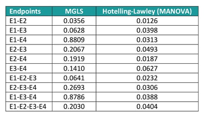
To illustrate how the GST could provide added value compared to standard multivariate approaches such as Multivariate ANOVA Hotelling’s T test, we’ve considered the MPTET dataset contained in the R package multcomp considering 4 endpoints and 2 treatments. In Table 2 and 3 and Figure 2 we have reported some basic univariate information, including pairwise correlations and ANOVA F tests. Whilst there seem to be some evidence that the treatment has indeed an effect on 3 out of 4 variables, the direction of the effect is not consistent, with E4 showing a decrease in Placebo compared to the active drug, unlike the other endpoints.
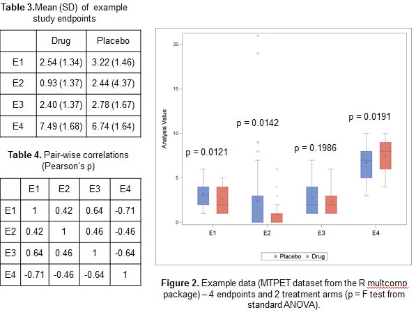
If new analyse all possible subsets of endpoints to identify the most promising ones, the Hotelling’s test returns significant results for nearly all combinations, whereas according to the MGLS test only E1 and E2 jointly are suggestive of a treatment effect (see table 5). The reason of this difference in results is that the Multivariate Analysis of Variance (MANOVA) approach only identifies ‘any’ difference, so that if two endpoints have a completely opposite direction, they would still jointly suggest a treatment effect even though the result is uninterpretable. The GST, on the other hand, assumes that the ‘benefit’ of one treatment versus the other has the same direction for all endpoints and as such only variables with e.g. a positive difference in the Active – Placebo comparison would be flagged as jointly significant.
Table 5: MPTET analysis example with GST and MANOVA techniques
Practical Considerations in GST
Statistical Power and Sample Size
Determining the sample size for the GST requires understanding the correlation structure among endpoints and ensuring sufficient statistical power. Each endpoint contributes to the overall power, and a high correlations may either inflate or reduce the power depending on the effect direction. Researchers often rely on simulation studies or advanced sample size calculators designed for multivariate data to obtain reliable estimates.
Handling Missing Data
Missing data can severely impact the robustness of the GST analyses. Techniques such as multiple imputation, which replaces missing values with predictions based on observed distributions, or complete case analysis, which uses only fully observed data, can be applied. However, it is crucial that these methods align with the underlying missing data mechanism – whether data are missing completely at random (MCAR), missing at random (MAR), or missing not at random (MNAR) – to avoid bias.
Software Implementation
The GST is computationally intensive and often implemented using specialised software like R and SAS, which provide flexible tools for multivariate testing tools.In R, the ICSNP package supports Hotelling’s T2 tests, the multcomp package facilitates multiple comparisons, and custom scripts can leverage matrix operations to manage correlations and endpoint weights. In SAS, PROC MIXED accommodates the covariance structure of multiple endpoints, and SAS macros simplify implementation in large-scale clinical trials.
While these considerations guide effective implementation, it's also important to be aware of areas where the GST can struggle.
Common Pitfalls and Limitations
Whilst the GST offers numerous advantages, there are a few caveats to keep in mind.
Assumption of Consistent Effect Direction
The GST works best when all endpoints are expected to move in the same direction (e.g. all improve or all worsen). When endpoints differ in direction, the global test may lose interpretability.
Excessive Correlation or Lack of Correlation
Whilst the GST utilises correlation, extremely high correlation between endpoints can inflate certain effects, whereas endpoints with very low correlation might not benefit from the global approach.
Complexity with Many Endpoints
As the number of endpoints grows, managing variance-covariance structures becomes more demanding, and interpreting a single global test can be more challenging.
Sensitivity to Missing Data
Missing data can distort results if not handled properly, especially in rank-based methods where complete data are typically required.
Overlooking Clinical Relevance
A global p-value alone does not indicate which individual endpoints drive the result. It remains important to interpret the clinical significance of each endpoint alongside the global effect.
Conclusion
Even with these considerations, the GST still offers a powerful, unified framework for addressing multiple endpoints in clinical trials when used judiciously. By leveraging correlations among endpoints, it reduces the risk of Type-I error inflation while preserving power, which is particularly important when outcomes conflict or vary widely in importance. Compared to traditional methods, the GST maintains the integrity of individual endpoints and can be applied across various data types, making it especially valuable in multifaceted diseases such as Parkinson’s. When coupled with standard multiplicity corrections, the GST further strengthens evidence of a meaningful overall treatment effect. With adaptable software options in SAS and R, researchers can implement the GST efficiently, ensuring both rigorous statistical control and clinically relevant insights for decision-making.

Quanticate's Statistical Consultants are among the leaders in their respective areas enabling clients to access specialised expertise tailored to your project requirements. To learn more about these services, please request a consultation below and a member of our Business Development team will contact you promptly.
References
- O’Brien PC. Procedures for Comparing Samples with Multiple Endpoints. Biometrics 1984; 40(4): 1079 - 1087
- Tang DI, Geller NL, Pocock SJ. On the design and analysis of randomized clinical trials with multiple endpoints. Biometrics 1993; 49: 23-30
- Dmitrienko A, Molenberghs G, Chuang-Stein C, Offen W. Analysis of Clinical Trials Using SAS – A Practical Guide. Cary, NC: SAS Press; 2007.


