Back to Blog

Delayed-entry models using PROC PHREG in Survival Analysis

By Statistical Consultancy Team | September 16, 2016

Delayed-entry_models_using_PROC_PHREG_in_Survival_Analysis.jpg

Time-to-event data often arise in clinical research, and in many cases represent the primary outcome of interest. These data generally represent the elapsed time between a reference time-point (e.g., treatment randomization) and an event of interest (e.g. death, relapse, etc.).

Whereas right censoring is a feature that is easily accommodated by most existing software, the same doesn’t strictly hold for another feature of survival data, left-truncation. In this post we’ll describe what left-truncation is, when it can arise and provide some SAS code that can be used to derive survival estimates and curves.

Left-truncation: causes and consequences

Let’s assume we’re running an observational study: subjects are enrolled in the study at time t if they’re either diagnosed with disease at the screening visit which occurs at time t itself or have already been diagnosed in the past. Suppose now that our main goal is to assess the overall survival from diagnosis, and that, for descriptive purposes, only right censoring occurs: if we were to include the subjects diagnosed prior to study entry in the risk set from the exact time when they were diagnosed, we would get biased survival estimates because we would not be considering the risk set of those subjects who were diagnosed prior to the study, but died before being enrolled in the study (and for which no information is thus available). As a result, we would be getting positively biased survival estimates.

To deal with this, subjects who have been diagnosed prior to study entry are not considered as being in the risk set until they’re actually enrolled in the study, i.e. their entry in the risk set is ‘delayed’. By doing this, we ensure that the subjects in the same year of re-mapped follow-up are comparable and survival estimates are not biased.

Accounting for this feature is not possible within PROC LIFETEST, but it can be done using some specific options in PROC PHREG. In the following section we present some SAS code and show the effects of not taking into account left truncation in cases when it arises.

Implementation in SAS

1. The ENTRY = option

Left panel of Figure 1 displays the standard Kaplan-Meier curve, obtained using standard PROC LIFETEST code, in a situation where left truncation is ignored, returning a median survival time of 5.37 years (95%CI: 4.07 – 7.15). Right hand panel, on the other hand, is taking delayed entry into account, i.e. subjects do not enter the denominator of the K-M estimator until they’ve been enrolled in the study. The most obvious difference is that this second curve is much steeper, with a median survival time falling between 3.41 and 3.43 years (the procedure doesn’t return the estimate, but an approximation can be retrieved by looking in the output dataset), and this is due to the fact that in the early years from diagnosis we’ve now removed from the denominator all those subjects that were diagnosed but not yet enrolled, thus resulting in a reduced survival probability. To achieve this, we have used the ENTRY (or ENTRYTIME) option in proc phreg, as follows:

PROC phreg data = survdata;
model &timevar*&censor(1) =/ entry = del_entry;
output out = delayed survival = S;
RUN;

This option specifies the time elapsed between the starting of the observation period (in this case, diagnosis) and the starting of the study period (in this case, enrolment).

Figure 1. Left panel: Survival estimates from PROC LIFETEST (left truncation ignored); right panel: survival estimates from PROC PHREG (left truncation accounted with the entry = option).

2. Alternative methods

There are different ways to extract the survival estimates from the PROC PHREG output: one, as shown above, is by means of the OUTPUT statement, which returns a dataset where the survival function is returned for each observation in the original dataset. Another one, which allows some additional variables to be exported to a SAS dataset is the BASELINE statement, as shown below:

PROC phreg data = survdata;
by <strata>;
model &timevar*&censor(1) =/ entry = del_entry;
baseline out = estimages survival = survival stderr = SE lower = lower upper = upper / cltype = log method = pl;
RUN;

Using this alternative code we can extract not only the survival estimate itself, but also its standard error, as well as confidence intervals and influence statistics. One additional feature of the BASELINE statement is the covariate option, which allows to ‘predict’ the survival curve for given levels of an explanatory variable added in the MODEL statement. If covariates are specified in the model and the covariate option is not specified then survival curves for mean values (for continuous variables) or reference levels (for categorical variables) of the covariates are returned. The argument of this option is a dataset containing the covariate names and all relevant combination of values/levels for which we want to predict the survival curve:

Covariate 1	Covariate 2
Value 1	Value 1
Value 1	Value 2
Value 2	Value 1
…	…
Value x	Value 2

Table 1. Layout of the covariates dataset

An example code is as follows:

data covariates;
<strata> = 'Level 1'; output;
<strata> = 'Level 2'; output;
run;

proc phreg data = survdata;
model &timevar*censor(1) = <strata> / entry = del_entry;
baseline out = estimates covariates = covariates survival = survival stderr = SE lower = lower upper = upper / cltype = log method = pl;
run;

The results using the two methods are displayed in Figure 2. The two approaches clearly provide different results: the left panel provides estimates that are just the same as those that can be obtained from the OUTPUT statement dataset (the only difference being that estimates are provided only for observations where an event has occurred), with the addition of further useful information, as described above. On the other hand, the left panel provide ‘predicted’ survival curves for the covariates that are entered in the model and at the levels specified in the covariates dataset. This last feature is particularly useful when we want to have an idea of the survival trend at given values of a continuous covariate.

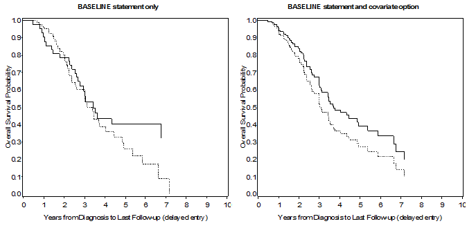
Figure 2. Left panel: Survival estimates from PROC PHREG, using a BY statement to get curves for different levels of a strata variable; right panel: survival estimates from PROC PHREG using the covariates = option in the BASELINE statement.

3. Potential Issues

As reported in a SAS support page [1], the usual product-limit estimator might provide meaningless estimates in some degenerate cases of left-truncation, e.g. when the first subjects entering the risk set either experience the event or are censored before any other subject enters the risk set. In this situation, the survival estimate would become 0 before some subjects actually start being at risk. As reported in [1], currently there’s no fix for this, and ad-hoc approaches will have to be implemented (e.g., exclude early events data).

CONCLUSION

In this post we have described what left truncated data are, when they can occur, and how they can be tackled using SAS software. See reference [2] for further reading on how to implement left truncation in SAS. The effect of not taking into account left truncation in a real context has been briefly described, and strategies to produce survival curves, both overall and for given levels of a ‘relevant’ covariate, using SAS 9.3 or later versions have been displayed.